Quang Vu
Chelsea Varella
Area of focus:
Sensor models (probability calculation)
Hypothesis:
We hypothesize that by changing the value of new_prob we will be able to improve the accuracy of the sensor particles/readings. In order to test our hypothesis we will test the current equation of ^3 against ^2, and ^4 in the update_particles_with_laser method.
Description of the measure (i.e. metric) used to evaluate the performance/success of the approach:
We will test three equations three times in three methods (nine times total) and record its success or failure:
-
The first method is to localize with minimal prior information (just the map of the environment). This will be referred to as "Normal Localization". For this method we will begin the robot in the upper left hand corner and direct it in a clockwise spiral towards the center.
-
The second method is maintain correct localization robustly in the face of frequent, complicated maneuvers. This will be referred to as "Complicated Maneuvers". For this method the robot will begin in the center and be randomly driven around.
-
The third method is if it is able to relocalize correctly after suddenly repositioned. This will be referred to as the "Kidnapped Robot". For this method the robot will be picked up and put in a new location within the boundries and randomly driven around.
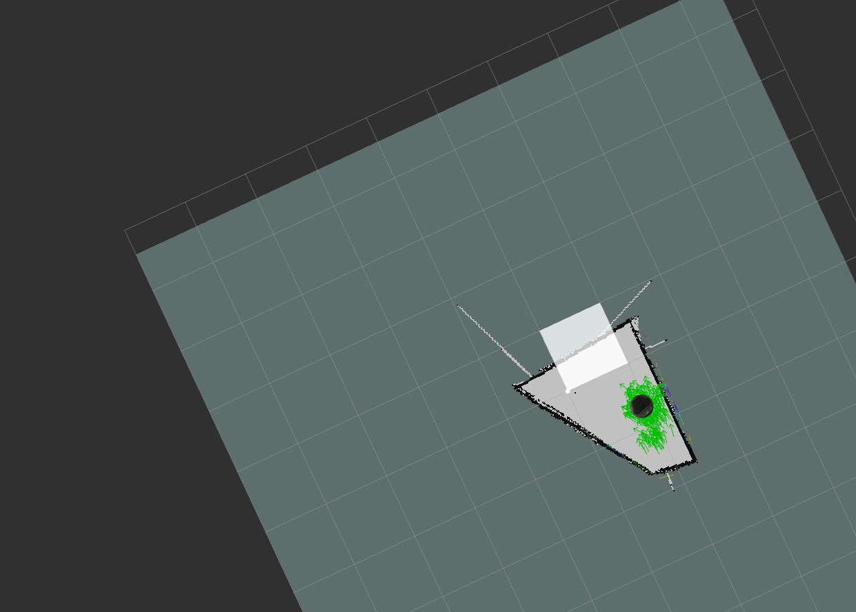
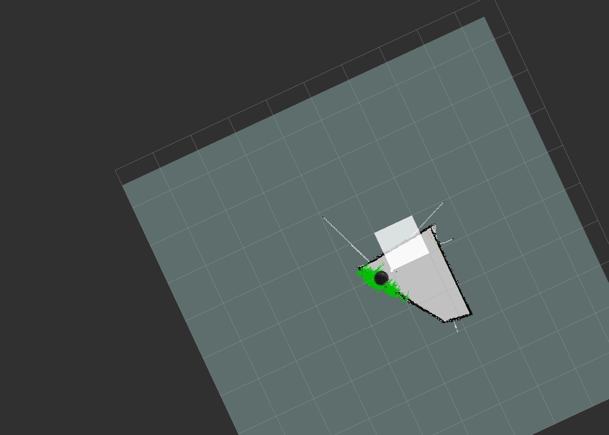
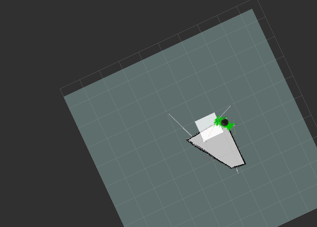
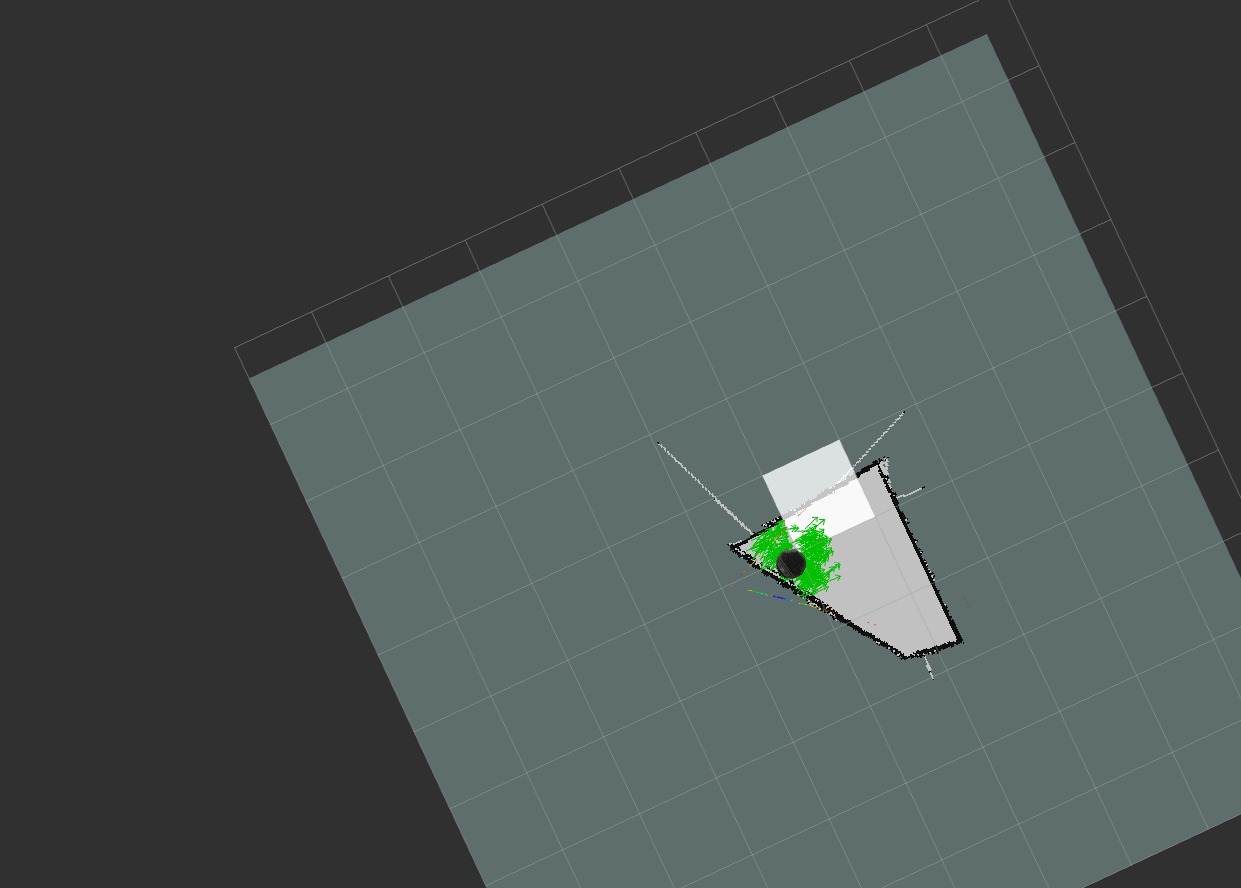
Success will be dependent upon the location of the robot on the map and the clustering and direction of the particles.
Map:

Data collected along with a description of how the data should be interpreted:
Trial One (Original (^3)):
Normal Localisation
Attempt 1: Success

Attempt 2: Success
Attempt 3: Failure

Complicated Maneuvers
Attempt 1: Success

Attempt 2: Success
Attempt 3: Success
Kidnapped Robot
Attempt 1: Failure

Attempt 2: Failure
Attempt 3: Failure
Trial Two (^2):
Normal Localisation
Attempt 1: Success
Attempt 2: Success
Attempt 3: Success
Complicated Maneuvers
Attempt 1: Success
Attempt 2: Success
Attempt 3: Success
Kidnapped Robot
Attempt 1: Close

Attempt 2: Failure
Attempt 3: Failure
Trial Three (^4):
Normal Localisation
Attempt 1: Failure

Attempt 2: Failure

Attempt 3: Failure

Complicated Maneuvers
Attempt 1: Success
Attempt 2: Success
Attempt 3: Failure
Kidnapped Robot
Attempt 1: Success

Attempt 2: Success
Attempt 3: Failure
Algorithms developed or modified:
Changing the value of new_prob calculation from def update_particles_with_lasedr(self, msg)
(Line 406 in pf.py)
Summary:
Even though the data is small, we can see a pattern of success and failure for each method of testing. Oddly enough, the more aggressive equation of ^4 did extremely well with the complicated maneuvers and the kidnapped robot scenario but did extremely poorly with the normal localisation. However, we need a bigger data sample in order to have a stronger conclusion.
Trial 1:
- Normal Localisation: 2 successes, 1 failures
- Complicated Maneuvers: 3 successes
- Kidnapped Robot: 3 failures
Trial 2:
- Normal Localisation: 3 successes
- Complicated Maneuvers: 3 successes
- Kidnapped Robot: 1 close, 2 failures
Trial 3:
- Normal Localisation: 3 failures
- Complicated Maneuvers: 2 successes, 1 failures
- Kidnapped Robot: 2 successes, 1 failures
For future students:
1. How to repeat:
Setup a small area similar to the map provided above.
For each calculation of new_prob:
- Normal Localization: place the robot in the upper left hand corner and direct it in a clockwise spiral towards the center.
- Complicated Maneuvers": place the robot anywhere on the map and drive around randomly to localize.
- Kidnapped Robot": pick up the robot and place it on a new location within the boundries and drive around randomly to localize.
- For each localiztion scenario, determine if localization is successful and record it. Take a picture of the current position of the robot and a screenshot of the map.
2. Apply the lessons and achieve the same peformance improvements:
The more aggressive calculation of ^4 seemed to work better for more complicated scenarios, however we did not have a very large data sample. Future students could also try even more aggressive calculations such as ^5 or ^6. Additionally, testing a larger sample set might have different results.
