CS 107 - Introduction to Scientific Computation Homework #10

1. Miniature Golf Simulation:  Imagine a 1 meter by 1 meter miniature golf green where

• you're putting (hitting the ball) from x = 0, y = 0, where the square green (playing area) goes from (0, 0) to (1, 1), corner to corner,
• the putt has initial velocity v, and initial angle theta in the range (0, pi/2) counter-clockwise from the x-direction looking down from the positive vertical (z) direction,
• there is a hole centered at (.5, .5) with a radius of .05,
• a ball within the hole radius drops in the hole and simulation stops,
• the square is tilted upward in the positive y direction, such that there is no acceleration in the x direction, and the y acceleration is -0.5 m/s/s,
• we will be ignoring the z coordinate, since we assume the ball will remain in contact with the ground,
• there are walls from (0, 0) to (0, 1), from (0, 1) to (1, 1), and from (1, 1) to (1, 0),
• these walls perfectly reflect the motion of the ball, causing the velocity to reverse in the direction perpendicular, and
• a ball that goes beyond the green (with negative y value) is out-of-bounds and simulation stops. Note: Do not solve for and terminate output with the point where y goes out of bounds.  The last x and y values returned are the first for which y < 0.

Create a function simGolf that takes as input:

• initial velocity,
• initial angle, and
• simulation time step

and returns as output:

• an integer that is -1 if the ball goes out of bounds, or the number of times the ball bounced off walls if the ball dropped in the hole,
• a vector of the simulation x values, and
• a vector of the simulation y values.

To simulate a bounce, do not merely reverse velocity, but also reflect the motion, such that the distance just traveled beyond a wall is reflected back as well.  For example, suppose you find that the y value is now 1.1.  This overshoots the wall by .1.  So the new reflected y value will now be 1 - .1 = .9. 

Within your simulation loop, the structure should be:

% change simulation value as if no walls exist
% in each case where a ball has gone beyond wall bounds, tally the bounce, reflect the motion, and reverse the velocity perpendicular to the wall
% add the new (x, y) point values to their respective result vectors.

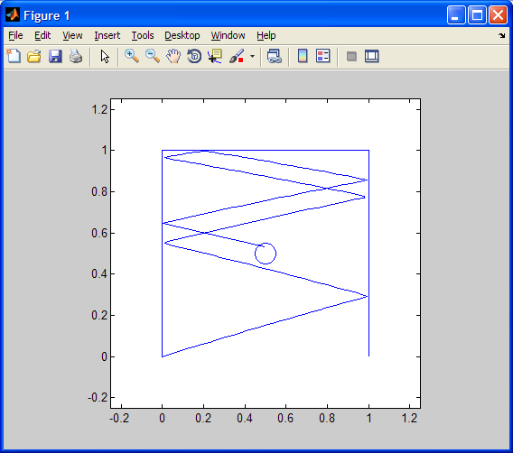
2. Plotting a Single Golf Simulation Trajectory:  Taking the same input as simGolf, your function plotGolf will

• use simGolf to simulate the golf ball trajectory,
• use "axis square" and axis limits from (-0.25, -0.25) to (1.25, 1.25),
• plot the golf ball trajectory,
• plot the walls,
• plot the outer edge of the hole or some approximation (see Exercise 3.5), and
• return the first output integer from simGolf.

For example, plotGolf(4, .3, .01) will return the integer 7 and plot this:

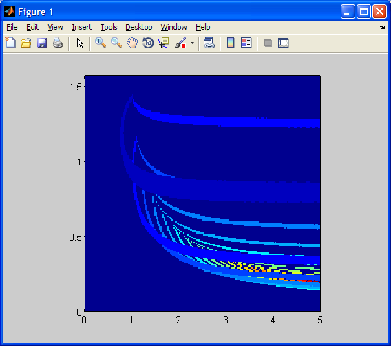
3. Plotting Many Golf Simulation Results: In function plotGolf2, you will take as input:

• the maximum initial velocity,
• simulation time step, and
• the number of points to linearly sample in each dimension of the simGolf input (initial velocity, initial angle)

The output will be the matrix of simGolf bounce count return values you will be plotting.

The initial angle theta will be in the range (0, pi/2).  The minimum initial velocity will be 0.  Use linspace, these bounds, and the number of points to sample to create a meshgrid of initial velocities and angles. For each initial velocity and angle, perform the simGolf simulation, and store the first return value in a matrix.  Finally, create a plot of the values using

pcolor(<initial velocities>, <initial angles>, <matrix of return values>);
shading('flat');
axis('square');

For example, plotGolf2(5, .01, 200) will return and plot this: