Homework #3
|
CS 107 - Introduction to Scientific Computation Homework #3 |
1. Polynomial: A polynomial is a function of the form c0 * x0 + c1 * x1 + c2 * x2 + ... + cn * xn. Since x0=1, this is equivalent to c0 + c1 * x + c2 * x2 + ... + cn * xn. All polynomial curve can be expressed in this form. The familiar line y = mx + b has n=1 with c1 being slope m and c0 being y-intercept b. A quadratic curve y = ax2 + bx + c has n=2 with c0, c1, and c2 being c, b, and a, respectively.
You will create a polynomial function "polynomial" in file polynomial.m that takes in (1) a scalar x, and (2) a vector coeff of coefficients (e.g. [c0 c1 c2]) and returns the y for that given polynomial. Note: The degree n of the polynomial is implicitly given by the length of the coefficient vector.
Example usage:
>> polynomial(7, [5])
ans =
5
>> polynomial(7, [5 2])
ans =
19
>> polynomial(7, [5 2 3])
ans =
166
2. Numerical Integration: While symbolic integration, the symbolic manipulation we learn in Calculus classes, is important and has valuable applications, there are many occasions where one is given raw data to integrate rather than a function. Given a function y = f(x), integration attempts to find the area underneath the curve over some interval. When one is given raw (x,y) values, a common simple method for integration is, for each adjacent pair of points, (xi, f(xi)) and (xi+1, f(xi+1)) to consider the trapezoid formed by these points and (xi, 0) and (xi+1, 0). A simple, good numerical integration approximation of the integral of a function can be formed by computing and summing the area of these trapezoids. Note: Area below the axis y = 0 is considered negative area.
For this exercise, we'll take a function sin(x) with a known integral function -cos(x), and compare the results of this trapezoidal numerical integration technique with the known correct results.
Begin by downloading the m-file called
trapezoidIntegrate.m. and follow
the implementation instructions therein.
From 0 to 1.5708 with step 0.1, the approximate area is 0.928488.
The actual area is 1, so the error is 0.0715117.

From 0 to 1.5708 with step 0.001, the approximate area is 0.999204.
The actual area is 1, so the error is 0.00079641.

From 0 to 1.5708 with step 1e-005, the approximate area is 0.999994.
The actual area is 1, so the error is 6.3268e-006.
3. Numerical Differentiation: Differentiation is the process of computing the rate of change, or slope, of a function. In cases where we are given a function that has no simple symbolic differentiation, we can turn to numerical differentiation.
Imagine you are standing at a point on a mountain slope, and you wish to measure the slope where you're standing. A single point altitude doesn't help. However, suppose you take an accurate altitude reading both one small step uphill and one small step downhill. By dividing the rise (change in altitude between the steps) by the run (distance horizontally between the two steps), we gain a good estimate for the slope where you're standing.
This analogy describes the simple three-point estimation method. Given an x value, a function f(x), and a small step h, one can estimate the derivative (i.e. slope) of f at x as (f(x + h) - f(x - h)) / (2 * h).
For this exercise, we'll again take the function sin(x) with a known derivative function cos(x), and compare the results of this numerical differentiation technique with the known correct results along a sequence of points.
Begin by creating a function called simpleDifferentiate.m.
Function simpleDifferentiate will take dx and h as parameters (in
that order). It will return the greatest (maximum absolute) error. First, assign values to a set of
variables:
xMin = 0; % minimum x test value
xMax = 2 * pi; % maximum x test value
x = xMin:dx:xMax; % x test values
Next, compute a vector of y values for sin(x).
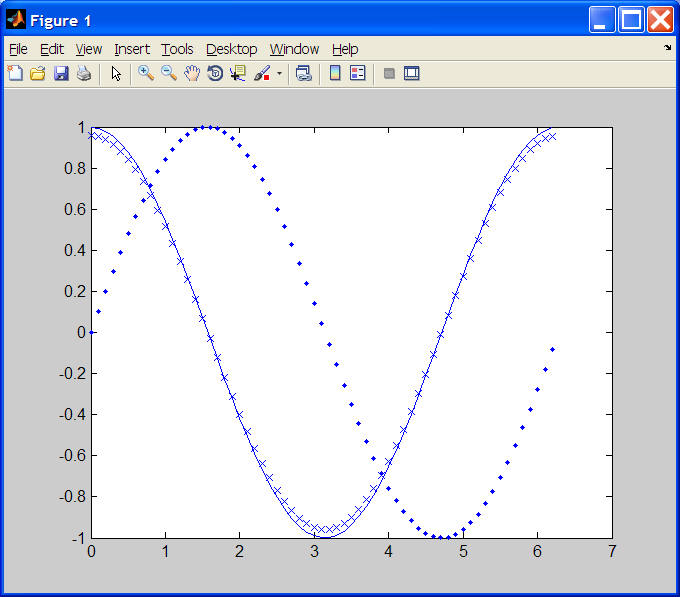
Plot x versus y as dots and hold the graph output.
Compute estimates and exact values for the derivative (cos(x)) at each x test
value, plotting each with "x" marks and lines, respectively. An example
plot for the variable values above appears below.
Finally, compute the maximum absolute error in the estimation, and display the
following output (with <placeholders> substituted with values):
From <xMin> to <xMax> with step <dx>, we numerically differentiate with h = <h>.
The greatest error is <maximum absolute error> at x = <x value for maximum absolute error>.
For example, here is the output of three m-file executions with dx = .1 and h assigned .5, .05, and .005, respectively.
From 0 to 6.28319 with step 0.1, we numerically differentiate with h = 0.5.
The greatest error is 0.0411489 at x = 0.
From 0 to 6.28319 with step 0.1, we numerically differentiate with h = 0.05.
The greatest error is 0.000416615 at x = 0.
From 0 to 6.28319 with step 0.1, we numerically differentiate with h = 0.005.
The greatest error is 4.16666e-006 at x = 0.