
Homework #3
|
CS 371 - Introduction to Artificial Intelligence
Homework #3 |
Important: To avoid loss of points, remove/comment-out unspecified printing from your code before submission. You would not believe how those best/current energy lines in SLS really add up in the log files.
1. Rook Jumping Maze Generation:
Rook Jumping Maze Instructions: Starting at the circled cell in the upper-left corner, find a path to the goal cell marked “G”. From each numbered cell, one may move that exact number of cells horizontally or vertically in a straight line. How many moves does the shortest path have?
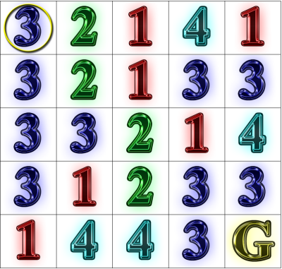
For this exercise, you will generate random n-by-n Rook Jumping Mazes (RJMs) (5 ≤ n ≤ 10) where there is a legal move (jump) from each non-goal state. You will also use stochastic local search to optimize for (1) solvability and (2) maximum length of the shortest maze solution path.
Let array row and column indices both be numbered (0, ..., n - 1). The RJM is represented by a 2D-array of jump numbers. A cell's jump number is the number of array cells one must move in a straight line horizontally or vertically from that cell. The start cell is located at (0, 0). For the goal cell, located at (n - 1, n - 1), let the jump number be 0. For all non-goal cells, the randomly generated jump number must allow a legal move. In the example 5-by-5 maze above, legal jump numbers for the start cell are {1, 2, 3, 4}, whereas legal jump numbers for the center cell are {1, 2}. In general, the minimum legal jump number for a non-goal cell is 1, and the maximum legal jump number for a non-goal cell (r, c) is the maximum of n - 1 - r, r, n - 1 - c, and c. This defines a directed graph where vertices are cells, edges are legal jumps, and the outdegree is 0 for the goal cell vertex and positive otherwise.
There are many features of a good RJM. One obvious feature is that the maze has a solution, i.e. one can reach the goal from the start. One simple measure of maze quality is the minimum number of moves from the start to the goal. For this exercise, we will limit our attention to these two measures of maze quality.
Using breadth-first search, or some other suitable graph algorithm, compute the minimum distance (i.e. depth, number of moves) to each cell from the start cell. Create an objective function (a.k.a. energy function) that returns the negated distance from start to goal, or a large positive number (use 1,000,000) if no path from start to goal exists. Then the task of maze generation can be reformulated as a search through changes in the maze configuration so as to minimize this objective function.
Implement stochastic local search state RookJumpingMaze according to this specification. Note that the specification of implemented interface methods is listed towards the top of the RookJumpingMaze documentation.
Once you have RookJumpingMaze implemented, complete the implementation of RJMGenerator.java. For a size 5 RJM, you should be able to implement and tune the parameters of a stochastic local search algorithm of your choice to achieve a median energy of less than or equal to -18.0 in 5000 iterations of search or less. That is, your median-energy maze generated should require a minimum of 18 moves to solve.
Hint: When computing the energy() method, you should not use your previous uniformed search code. Instead, coding a simple breadth-first search within the RookJumpingMaze class will allow you to easily do repeated-state elimination. Initialize the depth of the initial location to 0, and all others to a negative constant representing "unreached" status. Replace "unreached" values with search depths (one greater than current depth) as child locations are being added to the queue, and not adding children to the queue that have already been visited (have non-negative depth).
2. Distant Sampling: In many different problem, it is useful to be able to select a biased sample from a data set such that the items are very different from each other. Examples include initialization of clustering algorithms, choosing a color palette where colors are well distinguished from one another, and choosing sites to geographically distribute resources.
For this problem, you will create a stochastic local search State implemented according to this specification. Note that the specification of implemented interface methods is listed towards the top of the DistantSamplerState documentation. To summarize, the state is constructed with a 2D array where each row is an n-dimensional double point/vector, and a given number of distant samples from among these is the objective. Thus, to compute the energy, one computes the inverse squared Euclidean distance for each pair of points and sums these to get the "energy" of the State. To compute the Euclidean distance, compute the sum of the squared differences in each dimension between two points/vectors and then take the square root of this sum. To get the inverse squared Euclidean distance, you divide one by the distance squared. (Alternatively, don't take the square root when computing the distance and directly compute the inverse (i.e. reciprocal) without squaring. The square root and squaring are inverse operations and cancel.) It is as if we're simulating electrostatic rupulsion forces between our selected sample data points.
A stochastic local search step here is switching from one unique sample choice (no repetitions are allowed) to a different unique sample choice. It is convenient to internally represent our sample choices as a list of row indices from the original given data. More details to more methods are given in this specification.
Once you have DistantSamplerState implemented, complete the implementation of DistantSampler.java. For the default dataset given therein, you should be able to implement and tune the parameters of a stochastic local search algorithm of your choice to achieve a median energy of less than 132.0 in 10000 iterations of search or less.
Common problems and solutions:
Hopefully, in looking at these problems, you'll see the wide applicability of such optimization algorithms. Often, the most challenging aspect of such optimization is devising a good, efficient next state generator that gives beneficial structure to the state space, rather than merely bouncing randomly from one state to another. Good next state generators both allow one to traverse the entire state space, and immediately sample states that are similar in quality to the current state.