ISLR Weekly Assignments: Preparing Classification Data
 |
CS 371 - Introduction to Artificial Intelligence
ISLR Weekly Assignments: Preparing Classification Data |
You'll need this dataset: iris.csv
As we've seen already (and will see more of in chapters ahead), it is often a mistake to use all of one's data for learning, as we are prone to overfit our data. It is often wise to separate our data into training and testing sets. We train (i.e. regress, fit, learn classifiers, etc.) with one subset of data, and we test/evaluate the generalizing quality of that training against again a separate subset of data. In preparation for our classification tutorial, we will go through this process in R for the popular "iris" dataset. As a precursor to these steps, you should import the iris.csv in R as dataset "iris".
The first column of this dataset consists of irrelevant indices that should be omitted from our training/testing data:
> iris2 <- iris[-1] #remove first column
The last column consists of strings that are the target classes for our classifications. We need to convert these strings to factors for our classification task:
> iris2[,5] <- as.factor(iris2[,5]) #convert strings to factors for classification
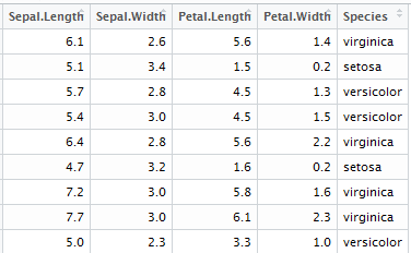
Eventually, we will split this data into 100 and 50 observations for training and testing, respectively. However, it would be unwise to split this data into the first 100 and last 50 as-is. Use the following command to view the data and see if you can understand why this is the case:
> View(iris2)
As you can see, the data is divided into equal classification groups of 50, so taking the first 100 for training would include all observations of 2 classes and none of the 3rd, and taking the last 50 for testing would include only those observations of the 3rd class for which we've had no training data! It would be beneficial to randomly permute or otherwise get a mix of all classes in both the training and the testing datasets. For our purposes, we will shuffle the data observations, but in order to all have the same ordering for our exercises, we will set the pseudorandom number generation seed to 0 before shuffling:
> set.seed(0)
> iris2 <- iris2[sample(nrow(iris2)),] #shuffle the rows

In practice, one often performs learning for different random samples or subsets of the data to see how sensitive performance is to the choice of training subset. Now examine the data ranges with the following command:
> summary(iris2)
Note how the data ranges vary. Sometimes, data ranges can vary by orders of magnitude, and some predictors can be seen as more significant to some algorithms simply because they take on greater magnitude values. A common step to prevent learning bias based on the magnitude of data ranges is to normalize the data, translating and scaling values so has to have the same ranges for each predictor. Perform the following steps to (1) define a column normalization function, (2) normalize our iris2 data so that all numeric predictor (columns 1:4) have the range [0, 1], and (3) verify that this has taken place:
> normalize <- function(x) { return ((x - min(x)) / (max(x) - min(x))) }
> irisnorm = cbind(as.data.frame(lapply(iris2[1:4], normalize)), iris2[5]) #convert numeric data ranges to [0,1]
> summary(irisnorm)
Note that this normalization doesn't imply that mean values are 0.5. (One might also perform a different normalization for data that is distributed normally where each predictor is translated and scaled so as to have a mean of 0 and a standard deviation of 1.)
We are now ready to partition our data into training and testing sets with corresponding classification labels:
> iris_train <- irisnorm[1:100,] #two-thirds training data
> iris_test <- irisnorm[101:150,] #one-third testing data
At this point, you are ready to perform the Moodle iris classification exercises. Of course, this preparation generalizes to working with other classification datasets.
Acknowledgements: This tutorial is derived in part from https://www.analyticsvidhya.com/blog/2015/08/learning-concept-knn-algorithms-programming/ which was originally written by Payel Roy Choudhury. My thanks to Payel and Analytics Vidhya.